
\( \def\bmatrix#1{\begin{bmatrix}#1\end{bmatrix}} \)
Matrix methods are a powerful tool in analyzing complex optical systems. Remarkably, any optical system, no matter how complicated, can be fully described by just four numbers, arranged in a two-by-two grid, which is called a matrix. This matrix of numbers lets us calculate where any paraxial ray will end up after it has passed through the system.
A matrix (plural: matrices) is a way of writing a set of linear equations. For example, if we have two linear equations,
these can be written in matrix form as:
It might seem a bit odd to write two equations this way, but matrix notation turns out to be very useful. In particular, matrices can be used to describe transformations of things (like rays) which is how they are used in optics.
One thing that mathematicians are famed for is laziness. Why write something twice, when once will do. And why write something at all, when you can leave it out completely. The development of matrix notation can be understood as a drive to write as little as possible.
In the set of linear equations
the symbols \( \alpha \) and \( \beta \) are written twice. We could rewrite the linear equations so that we only write \( \alpha \) and \( \beta \) once, like so:
If we do this, we have to understand that writing the \( \alpha \) and \( \beta \) above the columns means that we should, when we have to, multiply every number in the column by the number floating at the top of it.
The \( + \) symbols are also repeated, but really are they even necessary? If we are dealing with sets of equations, we ought to just know that we add together the \( A\alpha \) and the \( B\beta \) and so on. So we could simply get rid of the \( + \) symbols, like so:
With this notation, it's understood that after you have multiplied the first column of numbers by \( \alpha \), and multiplied the second column of numbers by \( \beta \), that you add the results across the rows.
The next step, it turns out, is crucial to making this notation actually useful (although we won't see this until later in the chapter). Sets of equations are most commonly presented, at least in school, as a puzzle: you are given the values of \( x \) and \( y \) on the left hand side, and \( A, B, C, D \), and you have to work out the values of \( \alpha \) and \( \beta \). However, this is not how equations are always used. Often, a set of equations is describing a transformation, where we start with \( \alpha \) and \( \beta \) on the right hand side, and then work out the values of \( x \) and \( y \) from them.
The annoyance with the notation we have made so far is that \( x \) and \( y \) are written in a column, but \( \alpha \) and \( \beta \) are written in a row, even though they are sort of the same: that is, they are both pairs of numbers. While this might not deeply trouble most people, it did annoy the developers of matrix notation, so they decided to make one more change, and write the \( \alpha \) and \( \beta \) in a column, like \( x \) and \( y \) are:
Finally, just to keep everything tidy, they visually grouped the numbers \( A, B, C, D \) by putting brackets around them, did the same with \( x, y \) and \( \alpha, \beta \), and got rid of one of the \( = \) signs, to get:
The box of numbers \( A, B, C, D \) is called a matrix. The columns of numbers \( x, y \) and \( \alpha, \beta \) are called vectors. The way the equations are written now, it looks a tiny bit like the vector \( \alpha, \beta \) is being multiplied by the matrix \( A, B, C, D \) to produce a new vector \( x, y \) . In a very real sense that's actually what's happening, although because the multiplication process is quite complicated it doesn't act the same as, say, just multiplying together two numbers.
If you need to get used to the idea of multiplying matrices and vectors, the box below contains a simple matrix-vector calculator. If you type in values for the matrix and vector and hit the calculate button, you'll get a new vector of values.
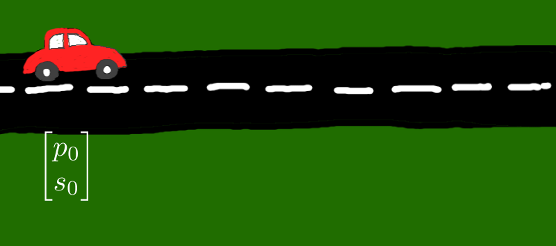
To see how matrices can be used to describe transforms, we'll take a little detour. Imagine a car driving along a straight road at a constant speed. At any time, we can describe the car by its position \( p \) and its speed \( s \). And if we know the position and speed of the car at any one time, we can easily work out its position and speed at a later time.
For example, suppose that at 12 o'clock, the car has a position of \( p=0 \)km and a speed of \( s=30 \)kph. A position equal to zero means the car is just starting out. After 1 hour, the position of the car is \( p=30 \)km, and the speed is (still) \( s=30 \)kph. After 2 hours, the position is \( p=60 \) km, and the speed is (still) \( s=30 \)kph.
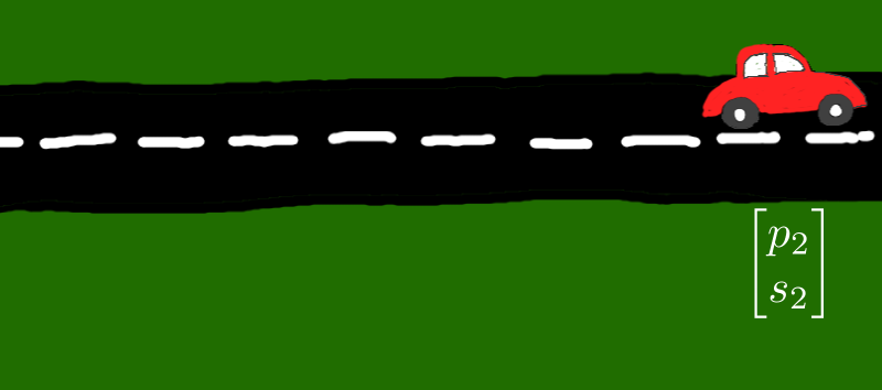
We're going to put all these facts into matrix notation now. Let's write \( p_0 \) and \( s_0 \) for the position and speed of the car at the start of the journey ( Figure 1(a) ). Let's write \( p_1 \) and \( s_1 \) for the position and speed of the car after 1 hour ( Figure 1(b) ), and \( p_2 \) and \( s_2 \) for the position and speed of the car after 2 hours ( Figure 1(c) ). (If the car travels at the same speed, \( s_0=s_1=s_2 \)).
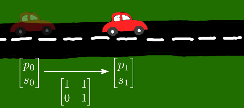
The position and speed at the start of the journey and after one hour can be related by a simple pair of equations, namely:
The first equation says that you calculate \( p_1 \) by starting with \( p_0 \) and then adding 1 hours worth of speed. The second equation just says the speed doesn't change. You can write this as a matrix equation ( Figure 2(a)):
Maybe from this you can see why the inventors of matrix notation wanted to write the pairs of numbers (the vectors) in exactly the same way. In this matrix equation, \( \bmatrix{p_0 \\ s_0} \) and \( \bmatrix{p_1 \\ s_1} \) really are the same kind of thing, namely a description of the position and speed of the car at different times, so it's good that they actually look the same in the equation.
The position and speed after 1 hour and after two hours can also be related by a simple pair of equations, namely:
Again, the first equation says that you calculate \( p_2 \) by starting with \( p_1 \) and then adding 1 hours worth of speed. The second equation just says the speed doesn't change. You can write this as a matrix equation ( Figure 2(a)):
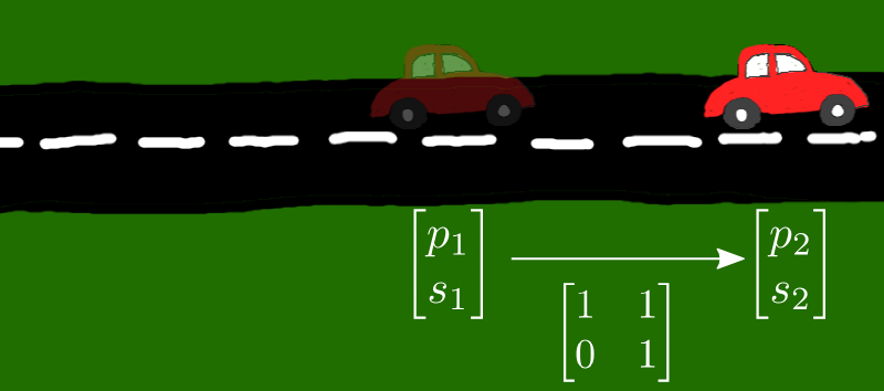
Notice that in the matrix equations (1) and (2), the matrix is the same. That matrix tells us how to transform the position and speed of the car at some time, into the position and speed of the car one hour later.
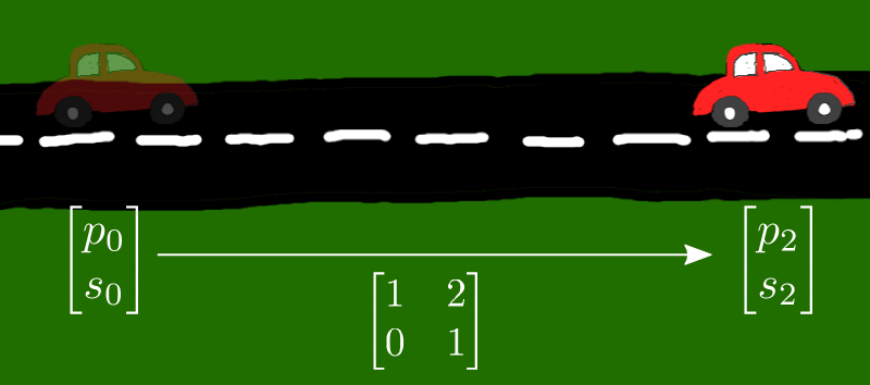
The position and speed at the start of the journey and after two hours can be related by a simple pair of equations, namely:
The first equation says that you calculate \( p_1 \) by starting with \( p_0 \) and then adding 2 hours worth of speed. The second equation just says the speed doesn't change. You can write this as a matrix equation ( Figure 2(c)):
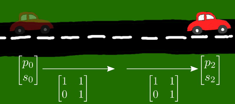
Now, this tells us that we can get the position and speed after two hours in two different ways: either by using Equation (3), or by using Equation (1) to work out the position and speed after 1 hour, and then use Equation (2) to get the speed after another hour ( Figure 3 ). These two ways ought to give the same answer, and of course they do. But more interestingly, they suggest that we can not just multiply a matrix and a vector together to get another vector (which is what we've been doing so far) but we can also multiply together two matrices to get another matrix.
Look at Equation (1). It tells us that \( \bmatrix{p_1 \\ s_1} \) is exactly the same as a matrix multiplied by \( \bmatrix{p_0 \\ s_0} \). So we could substitute the right hand side of Equation (1) into Equation (2) to give us:
Let's now assume that we can multiply matrices together and that it is associative, so we can rebracket this equation to give
If you compare this Equation (4) with Equation (3), you have to conclude that
So if we're using matrices to represent changes in the position and speed of a car, we have to be able to multiply them together to be consistent.
Luckily, if we know how to multiply a matrix and a vector, we know how to multiply two matrices. Here's how. Suppose we have to multiply together two matrices, like this:
The first step is to think of the second matrix as two vectors, side by side:
Next, because we know how to multiply a matrix and a vector, we take the two vectors of the second matrix, and write them out as separate multiplications:
\[\bmatrix{A & B \\C & D}\bmatrix{E \\ G}\]
|
\[\bmatrix{A & B \\C & D}\bmatrix{F \\ H}\]
|
Suppose the result of the multiplication on the left is:
We will write the result of the multiplication on the left:
\[ \bmatrix{W \\ X}\]
|
\[\bmatrix{A & B \\C & D}\bmatrix{F \\ H}\]
|
Suppose the result of the multiplication on the right is \( \bmatrix{Y \\ Z} \). Again, we write the result of the multiplication:
\[ \bmatrix{W \\ X}\]
|
\[\bmatrix{Y \\ Z}\]
|
Now we bring the two vectors back together:
and finally we write the two vectors as a single matrix by unsplitting them:
That is how you multiply matrices.
If you need to get used to the idea of multiplying matrices together, the box below contains a simple matrix-matrix calculator. If you type in values for the two matrices on the right and hit the calculate button, you'll get a new matrix which is the product of the ones on the right.
Note that matrices can be much bigger than a grid of four numbers, but this is the size that we use in optics (mostly).
The procedure we have worked out for multiplying two matrices is quite a lot more complicated than the procedure for multiplying two numbers. So you shouldn't be surprised that it doesn't act completely like regular multiplication. Regular multiplication is both associative and commutative. That is, for any three numbers, \( a(b c)=(a b)c \), and \( a b = b a \) .
Matrix multiplication is only associative. That is, if \( \mathbf{A} \), \( \mathbf{B} \), and \( \mathbf{C} \) are all matrices, then
\( (\mathbf{A} \mathbf{B} ) \mathbf{C} = \mathbf{A} (\mathbf{B} \mathbf{C}) \), so it's associative.
\( \mathbf{A} \mathbf{B} \ne \mathbf{B} \mathbf{A} \) usually, so it's not commutative, although sometimes it is.
The lack of commutativity makes it really crucial to write matrices in the right order when you multiply them.
There are a couple more things about matrix multiplication. First off, if you multiply a matrix by an ordinary number (which is called a scalar when there are matrices around), you just multiply all of its elements:
In ordinary multiplication, if you multiply anything by \( 1 \), it doesn't change it. There is a matrix which acts like \( 1 \) does, called the identity matrix:
For any matrix \( \mathbf{A} \), \( \mathbf{I} \mathbf{A} = \mathbf{A} \mathbf{I} = \mathbf{A} \). So, in this one instance, multiplication is commutative.
We finish up our introduction to matrices with the inverse matrix. In ordinary multiplication, every number \( n \) has an inverse \( 1/n \) so that when they are multiplied together, you get \( 1 \). For example, the inverse of \( 4 \) is \( 0.25 \). Only one number is missing an inverse, and that number is \( 0 \).
Matrices also have inverses. We define the inverse of a matrix \( \mathbf{X} \) as another matrix \( \mathbf{X}^{-1} \) which, when they are multiplied together, gives us the identity matrix \( \mathbf{I} \). That is,
Also, the inverse commutes:
It turns out that the inverse of a matrix with 2 rows and columns, like we use here, is really simple to define. If a matrix has elements \( A, B, C \) and \( D \), like this:
then it's inverse is simply
The number in front, \( 1/(AD-BC) \), is just a scalar, so we use the scalar multiplication rule above to work out the matrix. Not all matrices will have an inverse; if the term \( AD-BC \), called the determinant , is zero no inverse exists, because you can't divide by zero.
If a matrix \( \mathbf{C} \) is the product of two matrices \( \mathbf{A} \) and \( \mathbf{B} \) , \( \mathbf{C}=\mathbf{A B} \), then the inverse \( \mathbf{C}^{-1} \) is given by \( \mathbf{C}^{-1} = \mathbf{B}^{-1}\mathbf{A}^{-1} \). This is easy enough to show:
| Begin with: | \( \mathbf{C}\mathbf{C}^{-1} \) |
| Put in the definition of \( \mathbf{C} \) and the inverse: | \( (\mathbf{A B})(\mathbf{B}^{-1}\mathbf{A}^{-1}) \) |
| Use the associative law to change the brackets: | \( \mathbf{A} (\mathbf{B}\mathbf{B}^{-1}) \mathbf{A}^{-1} \) |
| Replace \( \mathbf{B} \mathbf{B}^{-1} \) with \( \mathbf{I} \) | \( \mathbf{A} \mathbf{I} \mathbf{A}^{-1} \) |
| \( \mathbf{A} \mathbf{I} = \mathbf{A} \) | \( \mathbf{A} \mathbf{A}^{-1} \) |
| Replace \( \mathbf{A}\mathbf{A}^{-1} \) with \( \mathbf{I} \) | \( \mathbf{I} \) |